Understanding the Value Function in Reinforcement Learning: A Corridor Example

Value functions are a fundamental concept in Reinforcement Learning (RL). A solid grasp of value functions is essential for understanding more advanced RL algorithms. In this post, we explore value functions through a simple, custom environment to make their core ideas intuitive and accessible. We also provide the python code to replicate our results here.

Deterministic Corridor Environment

Imagine a corridor divided into N discrete states. An RL agent navigates this corridor in search of an exit door. Initially unaware of the exit’s location, the agent must explore the environment.

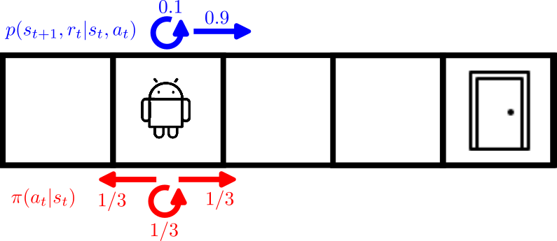
If the environment is stochastic, outcomes are uncertain. Specifically, from a given state \(s_t \in \mathcal{S}\) and action \(a_t \in \mathcal{A(s_t)}\), the next state is governed by a probability distribution. This uncertainty may be aleatoric (inherent randomness) or epistemic (lack of knowledge about the system).

The following must always hold for transition dynamics:

$$ \sum_{s_{t+1} \in \mathcal{S}} \sum_{r_t \in \mathcal{R}} p(s_{t+1}, r_{t}| s_t, a_t) = 1$$

\(p(\cdot)\) is the transition probability function or dynamics model. For instance, in a stochastic corridor, the agent might intend to move right but has a 10% chance of staying in place due to slippage.

In a deterministic environment, the agent’s action always results in a predictable next state.

Deterministic Policies

A policy \(\pi(a_t|s_t)\) defines the agent’s decision-making process. If deterministic, it maps each state to a single action:

$$a_{t} = \pi(s_t)$$

This means the agent always takes the same action from a given state.

What Is a State-Value Function?

In RL, by “value”, we mean the potential reward that the agent will get if it follows a given policy \(\pi\). The state-value function \(V_{\pi}(s_t)\) represents the expected total reward that the RL agent will get starting from state \(s_t\). The total reward takes the name of return \(G\) and it can be discounted in the case of continuing tasks. The discount factor “gamma” \(\gamma \in [0,1]\) accounts for the fact that immediate rewards are more valuable than future rewards, as these are usually not guaranteed. More formally, the return \(G\) is defined as [1]:

$$ G_t = R_{t+1} + \gamma R_{t+2} + \gamma^2 R_{t+3} \dots \gamma^{T-1} R_T$$

Or compactly:

$$G_t = \sum_{k=t+1}^{T} \gamma^{k-t-1} R_k$$

The state-value function \(V_{\pi}(s_t)\) is defined as the expected return, therefore we can write:

$$V_{\pi}(s) = \mathbb{E}_{\pi}[G_t|S_t = s]$$

The operator \(\mathbb{E}_{\pi}\) tells us that this is the expectation under a given policy \(\pi\). We can see here already that the value depends on a policy. If the policy is “good” and leads the agent to the goal (for example, the door in our corridor example) then the value will be higher in a given state \(S_t = s\).

The Bellman Equation

It is important to highlight the recursive nature of the value-function. As a matter of fact, we can show that:

$$G_t = R_{t+1} + \gamma G_{t+1}$$

This means that the return can only be computed analytically for episodic environments. In such scenarios we have access to the terminal state T and we can iterate backwards from T to t. This often not practical and it is much more common to use estimates of the return that do not require waiting till the end of an episode to update the returns of the all trajectory. This is one of the core equations of dynamic programming which enables online learning and using RL in continuing tasks where there is no terminal state.

Similarly, if we expand the definition of the expectation \(\mathbb{E}_{\pi}\) we get the definiton of the state-value function in recursive form:

$$ V_{\pi}(s_t) = \sum_{a_t \in \mathcal{A(s_t)}} \pi(a_t|s_t) \sum_{s_{t+1} \in \mathcal{S}} \sum_{r_t \in \mathcal{R}} p(s_{t+1}, r_t| s_t, a_t)[r + \gamma V_{\pi}(s_{t+1})] $$

The equation above is the Bellman equation for \(V_{\pi}(s_t)\) and it represents one of the cornerstones of dynamic programming and reinforcement learning. In the next section, we will dive deeper into this equation and we will learn how to apply it to our corridor environment.

How to Compute the State-Value Function

If we restrict the scope of the equation above only to the deterministic corridor environment we can get a simplified version of the Bellman equation which can be useful to understand some of its basic properties. In the deterministic case \(p(s_{t+1}, r_{t}| s_t, a_{\pi}) = 1\) where \(a_{\pi}\) is the action taken by the policy \(\pi\) and \(p = 0\) for all the other possible actions in \(\mathcal{A}(s_t)\). This means that we can simplify the Bellman equation to:
$$ V_{\pi}(s_t) = \sum_{a_t \in \mathcal{A(s_t)}} \pi(a_t|s_t) [r + \gamma V_{\pi}(s_{t+1})] $$

Moreover, for a deterministic policy \(\pi(a_t|s_t)= 1\) if \(a_t = \bar{a}\) and \(\pi(a_t|s_t)= 0\) otherwise. In this case, the state-value function can be expressed as:

$$ V_{\pi}(s_t) = r + \gamma V_{\pi}(s_{t+1}) $$

We will now see three different ways of finding the value function for a fixed policy. We will use the same policy for all the different methods, in particular we will assume that the agent starts from the left of the corridor and moves to the right at every step until it find the exit door (which is placed all the way to the right).

1. Analytical State-Value Function Computation

Computing the value of a given policy is often referred to in the reinforcement learning community as the prediction problem [1]. This is opposed to the problem of improving the policy, referred to as control problem.

In the tabular case, it is possible to compute the state-value function analytically using matrix algebra. We can factor the terms into the following matrices \(P_{\pi} \in \mathbb{R}^{||\mathcal{S}|| x ||\mathcal{S}||}\) and \(R_{\pi} \in \mathbb{R}^{||\mathcal{S}||}\):

$$ P_{\pi} = \sum_{a_t \in \mathcal{A(s_t)}} \pi(a_t|s_t) \sum_{s_{t+1} \in \mathcal{S}} \sum_{r_t \in \mathcal{R}} p(s_{t+1}, r_t| s_t, a_t) $$

$$ R_{\pi} = P_{\pi} \cdot R(s_t, a_t)$$

where \(R(s_t, a_t) \in \mathbb{R}^{||\mathcal{S}||}\) is a vector containing all the values \(r_t\) in its elements. We can then factorize the Bellman equation in the following way:
$$V_{\pi} = R_{\pi} + \gamma P_{\pi} V_{\pi} $$

We can then invert the equation above and we get:

$$V_{\pi} = (I – \gamma P_{\pi})^{-1}R_{\pi} $$

2. Policy Evaluation

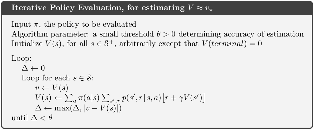
Policy evaluation is a recursive method to estimate the value of a given policy. Unlike the analytical method, it’s a very generic method that can be applied to any Markov Decision Process (MDP), not just the tabular case. Its generality is what makes it one of the pillars of reinforcement learning. You can find the algorithm here below as described by Sutton et al. [1].

You can find the code for both the analytical computation and the iterative policy evaluation method in our Github page. Here below is a snippet of our code showing the Python implementation.

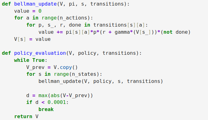
By running the Jupyter notebook, you will see that in case of a deterministic policy the final solution for the state-value function using the iterative method is the same as the one we found with the analytical method above. The iterative approach, however, is better suited to online learning where the algorithm doesn’t need to recompute the whole value function at every interaction with the environment, but it can only update the entry of the state it visits.

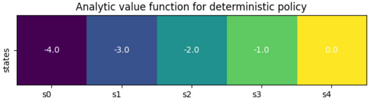
We can see clearly from Fig. 4 that the entries of the state-value function for a policy that is deterministically moving right, represent how far the agent is from the goal. As a matter of fact the state-value in state \(s4\) is exactly zero as the agent has already reached the goal. If the agent is instead in state \(s0\) then it will take it at least 4 steps to reach the goal at \(s0\) and it will accumulate a reward of -1 at each step, thus reaching a total penalty of -4. This is only true for episodic tasks where the environment stops once the agent reaches the goal and, by definition, the value of the terminal state \(V_{\pi}(s4)\) is zero.

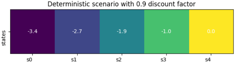
The figure above portrays the same deterministic corridor scenario as Fig. 4 above, using this time a discount factor \(\gamma\) of 0.9. You can see the effect of this factor on the entries of the state-value function that are further away from the goal. In this Jupyter Notebook you can go further into this topic and see how the discount factor plays a key role in those environments with sparse rewards and where the reward function has no in-built time penalization.

Stochastic Case

The task can be stochastic because the policy isn’t deterministic, because the environment is stochastic (i.e. the corridor is slippery), or both. We show here below what the value function can look like in the fully stochastic case (same as the one shown in Figure 1 above).

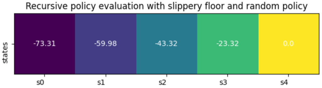
Intuitively, we can see explain how the value of \(s0\) is much lower than in the deterministic case: the agent has to take many more steps to reach the goal as it slips while it tries to move to right towards the goal. Instead of just taking 4 steps, it might have to attempt dozens of steps thus accumulating a much lower return.

Conclusion

• The state-value function \(V_{\pi}(s)\) can be seen as a measure of the total return that can be achieved from the state \(s\) following the fixed policy \(\pi\);
• The state-value function \(V_{\pi}(s)\) can be computed analytically under the following conditions:
  • the tabular case (discrete states and actions spaces);
  • the policy \(\pi\) doesn’t change;
  • the model / transition dynamics is known and is stationary (i.e. doesn’t change).
• The iterative policy evaluation is better suited to online/real time learning methods where we don’t need to update the whole value-function before taking a new action.

Visit this Jupyter Notebook to find the code used to generate the images above and to see more how the environment setup and reward function affects the value function. We encourage you to fork the repository and experiment with your own environment parameters and reward functions!

Code

• You can find a Jupyter Notebook with all the python code and instructions to replicate the results above at this GitHub link.

References

• [1] R. S. Sutton and A. G. Barto, “Reinforcement Learning“, 2nd edition, 2015;
• [2] Fundamentals of Reinforcement Learning, Martha White and Adam White, visited Feb. 2025.