Value Estimation with Monte Carlo Methods: Learning from Experience

We are now going to tackle for the first time the challenge to determine the value function when we don’t have access to a model. This will be very useful to move on to more complex environments where the interactions are much more complex than the Corridor example we have been working with so far.

If you haven’t seen the previous blog posts on Value function in Reinforcement Learning and on the Generalized Policy Iteration (GPI), go check them out. In those posts you will find an introduction to the corridor example and to model-based value estimation using Dynamic Programming. That strategy requires the agent to have full knowledge of the environment’s dynamics, specifically, the transition probabilities \(p(s’, r | s, a)\).

But what happens when the agent doesn’t have a map of the world? In this post, we introduce Monte Carlo (MC) methods. Unlike DP, Monte Carlo methods are model-free; they allow an agent to estimate the value of states simply by interacting with the environment and averaging the returns actually received.

Recap: The Corridor Environment

To demonstrate this, we are using the CorridorEnvTerminalReward environment from our source code. Here is how it differs from our previous examples:

• Sparse Rewards: Unlike the previous corridor where the agent got \( -1\) at every step (a “time penalty”), here the reward is 0.0 for every transition except when reaching the goal.
• The Big Prize: When the agent reaches the terminal state (the door at the far right), it receives a +10.0 reward.
• The Logic: In this world, “time is free,” but the “goal is everything.”

How Monte Carlo Estimation Works

The core idea of Monte Carlo is simple: Value is the average return.

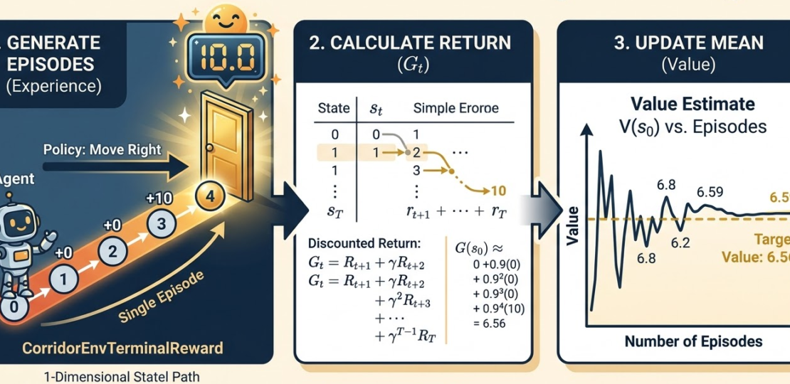
In DP, we used the Bellman equation to “bootstrap,” meaning we updated the value of a state based on the estimated value of the next state. In Monte Carlo, we don’t bootstrap. Instead, we play out an entire episode from start to finish, calculate the total return \(G_t\), and then update our estimate.

The Algorithm: First-Visit MC

1. Generate an Episode: Follow the policy \(\pi\) until the agent reaches the terminal state (the door). Record the sequence of states and rewards: \(S_0, R_1, S_1, R_2, \dots, S_T\).
2. Calculate Returns: For each state \(s\) visited in the episode, calculate the return \(G_t = \sum_{k=t+1}^{T} \gamma^{k-t-1} R_k\).
3. Average: Keep a running average of the returns received for each state across many episodes.

Mathematically, as the number of episodes \(n \to \infty\):

$$V_{\pi}(s) \approx \frac{\sum_{i=1}^n G_{i}(s)}{n}$$

From GPI to Monte Carlo: Comparing the Results

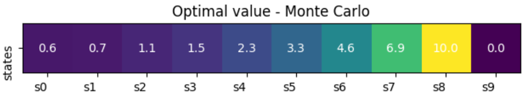
In our GPI post, we showed that by iteratively applying policy evaluation, the value function \(V(s)\) converged to a specific set of numbers. For a 10-state corridor with a deterministic “move right” policy and \(\gamma = 0.95\), the values were:

• \(V(s_0) = 0.4\)
• \(V(s_1) = 0.6\)
• \(V(s_2) = 0.8\)
• \(V(s_n) = …\)
• \(V(s_8) = 10\)
• \(V(s_9) = 0\) (terminal state)

When we run the Monte Carlo Python implementation, we observe something fascinating: the results are identical. You can compare this result to the one obtained in the “Discounted Case with Terminal Reward” in this notebook.

Why do they match?

Even though the mechanisms are different (one uses a mathematical model of the world and the other uses “brute force” experience) they are both estimating the same underlying property: the Expected Return.

Because the Corridor is a stationary MDP, the law of large numbers ensures that our Monte Carlo averages will eventually converge to the exact values defined by the Bellman Equation. The primary difference is that Monte Carlo requires the agent to actually “live” through the episodes, making it ideal for complex environments where the physics or rules are too complicated to write down as a probability matrix.

Conclusion

Monte Carlo methods show us that we can learn the value of our actions through pure experience. While it may require many episodes to converge compared to the surgical precision of Dynamic Programming, it frees us from the need for a perfect model of the environment.

In our next post, we will look at Temporal Difference (TD) learning, which combines the best of both worlds: the model-free nature of Monte Carlo with the efficiency of bootstrapping from DP.