Bayes’ Theorem and its Applications to Classification and Sequence Models

Bayes’ Theorem and the Naïve Bayes classifier are foundational concepts in probability and machine learning. But what do they mean in practical terms? Let’s break it down with a simple example.

Imagine you’re walking through the streets of Berlin and a stranger smiles and says “ciao!”. Naturally, you might wonder: Is this person Italian? Or could it be a local Berliner casually using an Italian greeting?

At first, your prior belief might suggest that the person is Italian—after all, “ciao” is an Italian word. And given the high number of Italian tourists and residents in Germany, that wouldn’t be an unusual conclusion. But think again: “ciao” (or “tschau”) is also widely used in Germany as a casual goodbye. So, how much evidence does that word really provide?

This seemingly trivial scenario is a perfect way to introduce Bayesian inference. Using Bayes’ Theorem, we’ll explore how to update our beliefs in the presence of new evidence and how the Naïve Bayes algorithm applies this logic to data classification problems.

Background

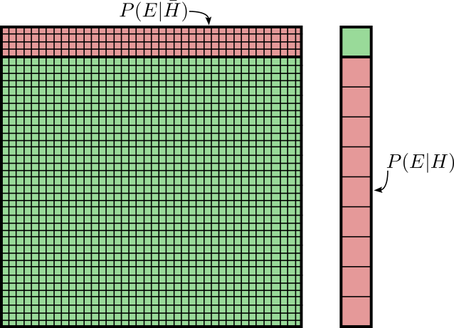
Consider your initial hypothesis \(H\) and the corresponding probability \(p(H)\). This would be the probability of a complete stranger in Berlin being Italian, this is called prior in Bayesian terminology. Consider then a probability \(p(E)\) of the event (or evidence) \(E\) of someone saying “ciao” in Germany occurring. The knowledge of \(p(E)\) gives us the chance to improve our knowledge of \(p(H|E)\), namely the probability of our random stranger being Italian considering that he used the Italian word “ciao”. Sometimes \(E\) is also called the data. \(p(H|E)\) is called the posterior in Bayesian jargon while \(p(E|H)\) is referred to as likelihood.

Using the language of joint distributions of random variables we define different types of probabilities:

• Joint probability \(p(H,E)\) = \(p(H{\cap}E)\) (probability of H “and” E) is the probability of two events \(H\) and \(E\) both occuring at the same time. In terms of sets theory this can be represented in a Venn diagramm as the intersection of the sets \(H\) and \(E\). In our example above this is the probability of an Italian using the word “ciao”;
• Marginal probabilities \(p(H)\) and \(p(E)\) express the total probability of an independent distribution, ignoring the possible cross correlations. \(p(H)\) (the prior) tells us how likely it is to find an Italian in Germany while \(p(E)\) (the evidence) tells us how likely it is for anyone to say “ciao” regardless of their nationality;
• Conditional probabilities \(p(H|E)\) (probability of H “given” E) expresses how the probability distribution H gets affected by a correlated event E, in our example this corresponds to how likely it is for a strager to say “ciao”, knowing that they are Italian. \(p(E|H)\), instead, represents the probability of a random stranger saying “ciao” given the fact that they are Italian.

Bayes rule

Bayes’ rule helps us improve our knowledge of the probability of a given distribution (the prior), given new information obtained through the event y. The rule states the following:

\begin{equation} p(H|E) = \frac{p(H,E)}{p(E)} = \frac{p(H{\cap}E)}{p(E)} \tag{1} \end{equation}

The conditional rule of probability tells us that \(p(H,E) = p(E|H) p(H) = p(H|E) p(E)\). We can use it to write Bayes’ theorem is a different form:

$$ p(H|E) = \frac{p(E|H)p(H)}{p(E)} \tag{2} $$

This is very useful whenever you want to invert a conditional probability and express the probability of “E given H” rather than “H given E”.

The law of total probability tells us that \(p(E) = p(E|H) p(H) + p(E|\bar{H}) p(\bar{H})\). We can use it to write the Bayes’ rule in one more form:

$$ p(H|E) = \frac{p(E|H) p(H)}{p(E|H) p(H) + p(E|\bar{H}) p(\bar{H})} \tag{3} $$

Equations (1), (2) and (3) are all different ways to express the Bayes’ rule and they can come handy in different situations.

Back to the Friendly Stranger Example

Let us now add some numbers to this example to see how it can be used in practice. We know that there are more or less 80 million people in Germany and 800 thousand of them are Italians. We also know that “ciao” is quite a common expression used by anyone in Germany and there is a 10% chance that a non-Italian speaker would actually use it in their every day life. What is the chance that a random stranger saying “ciao!” is actually Italian?

This means that:

• \(p(H) = \frac{8 \cdot 10^5}{8 \cdot 10^7} = 0.01 = 1\%\) is the probability of a random person in Germany being Italian;
• \(p(E|\bar{H}) = 0.1 = 10\% \) is the probability of a stranger greeting you with “ciao” when we know they are not from Italy;

We can then infer that \(p(\bar{H}) = 1 – 0.01 = 0.99\) is the probability of not being Italian in Germany. If we assume that pretty much every Italian will greet you with a “ciao” (\(p(E|H)=1\)) we then have everything we need to plug the numbers in the equation:

$$ p(H|E) = \frac{1 \cdot 0.01}{1 \cdot 0.01 + 0.1 \cdot 0.99}$$

$$ p(H|E) = \frac{0.01}{0.109} = 9\%$$

In conclusion, we can conclude that we have a \(9\%\) probability that the stranger who randomly greeted us with a “ciao” is Italian, even if we are in Berlin! Thanks to the Bayes’ theore have improved our prior \(p(H)\) and we have computed a posterior \(p(H|E) = 9\%\) which more accurately describes what we know.

Naïve Bayes Approximation

Let us make the example slightly more complicated now and let us also consider a number of other evidence that can contribute to our problem. For example the looks of the person might be relevant, or we may decide to ask their name. All these evidence contributes to our understanding of the problem and can be used further refine our prior knowledge.

Let us slighly change our naming and call the data in the following way:

• \(D_1\) is the friendly stranger greeting you with a “ciao”;
• \(D_2\) is the same person having mediterrean looks;
• \(D_3\) represents that same person having a seemingly Italian name.

Using the chain rule, we could plug all this information into the Bayes’ rule and we would get something like this:

$$ p(H|D_1{\cap}D_2{\cap}D_3) = \frac{p(H{\cap}D_1{\cap}D_2{\cap}D_3)}{p(D_1{\cap}D_2{\cap}D_3)} $$

The numerator can be expanded in this way using the chain rule:

$$ p(D_1|D_2{\cap}D_3{\cap}H) \cdot p(D_2|D_3{\cap}H) \cdot p(D_3|H) \cdot p(H) \tag{4} $$

As you can see this equation accounts for the correlation in the data. For example \(p(D_2|D_3{\cap}H)\) expresses the probability of a person having mediterrean looks (\(D_2\)) not just given them being Italian (\(H\)), but also given their name (\(D_3\)). Although correct, this makes the Bayes’ theorem much harder to apply, expecially when applied to classification problems where we may have thousands of data and considering each cross-correlation becomes untractable.

The naïve Bayes’ approximation consists in considering all the data conditionally independent. While this is only an approximation and is in general not true, it suddenly makes each term in the numerator of the Bayes’ theorem much easier to estimate:

$$ p(D_1|H) \cdot p(D_2|H) \cdot p(D_3|H) \cdot p(H) \tag{5} $$

In classification problems the goal is usually to perform Maximum Likelihood Estimation (MLE) to \(p(H|D_1{\cap}D_2{\cap}\dots{\cap}D_N)\). Because the denominator only depends on the data (and, therefore, it cannot be changed) it can be ignored and MLE can be applied directly to the equation above.

Sequence Models

Bayes’ theorem is also widely used in sequence models such as Natural Language Processing (NLP) applications like speech recognition, spelling correction and autocomplete. In this case the NLP algorithm is given a sentence as a sequence of words and needs to predict the next most likely candidate word. This is a different problem than the friendly stranger we discussed above where we had an hypothesis \(H\) and an event/evidencee \(E\), and we have instead a series of ordered words \(W_1, W_2, W_3 \dots W_M\). However, we can still apply the Bayes’ theorem to try and find the \(Mth\) most likely word given all the previous ones. In other words, we can use Eq. 1 to compute \(P(W_M | W_1, W_2, \dots W_{M-1})\):

$$ P(W_M | W_1, W_2, \dots W_{M-1}) = \frac{P(W_1, W_2, \dots W_{M})}{P(W_1, W_2, \dots W_{M-1})} \tag{6} $$

A common approximation for this is to consider only the relationship between a word and the N words before that. These are called N-Grams.

Like in the classification example the denominator of Eq. 6 is fixed we only need to optimize the numerator.

$$ P(W_1, W_2, \dots W_{M}) = P(W_1) \cdot P(W_2, \dots W_M | W_1) $$

Applying the chain rule:

$$ = P(W_1) \cdot P(W_2 | W_1) \cdot P(W_3 | W_2, W_1) \cdot \dots P(W_M | W_{M-1}, \dots W_3, W_2, W_1) \tag{7} $$

Using N=1, the N-Grams approximation results in the following equation:

$$ P(W_1, W_2, \dots W_{M}) = P(W_1) \cdot P(W_2 | W_1) \cdot P(W_3 | W_2) \cdot \dots P(W_{M} | W_{M-1}) \tag{8} $$

Equation 8 is much simpler than Eq. 7 as it ignores the dependencies between non-consecutive words in a sentence. Although this might be considered as a rough approximation, it leads to good results in multiple applications of series modeling.

Other practical examples

• Steve Brunton‘s video on the Medical Test Paradox;
• 3Blue1Brown example on Farmer and Librarian (inspired by Kahneman and Tversky);
• 3Blue1Brown‘s explanation of the Medical Test Paradox.

References

• ProbabilityCourse.com