Finding a Reinforcement Learning Policy with a Markov Decision Process: Generalized Policy Iteration (GPI)

How to find a policy when you have a model of your Markov Decison Process (MDP)? There is a number of methods to do this that all fall under the umbrella of Generalized Policy Iteration (GPI). Here we will go through the two most notable methods – Policy Iteration and Value Iteration – and we will see how to implement them in Python.

In this post we have already discussed what is the state-value function and how to compute for a simple example. In that case, the policy was fixed and we limited ourselves to evaluating the policy, not improving it. In this post we discuss instead how to obtain an optimal policy. The first step is to familiarize with the Bellman equations and with the concept of state-action value function.

State-Action Value Functions and Bellman Equation

The value of a policy is defined the expected return (i.e. the discounted total reward) that the agent will get if it follows a given policy. The state-action value function represents the expected total reward that the RL agent will get starting from state \(s_t\) and taking the action \(a_t\). This is, sometimes, also referred to as quality function, indicated by \(Q(s_t,a_t)\):

\begin{equation} Q_{\pi}(s_t, a_t) = \sum_{s_{t+1} \in \mathcal{S}} \sum_{r_t \in \mathcal{R}} p(s_{t+1}, r_t| s_t, a_t)[r + \gamma V_{\pi}(s_{t+1})] \tag{1} \end{equation}

The state value function \(V(s_t)\) and the state-action value function \(Q(s_t,a_t)\) are closely related by the following equation:

\begin{equation} V_{\pi}(s_t) = \sum_{a_t \in \mathcal{A(s_t)}} \pi(a_t|s_t) Q_{\pi}(s_t, a_t) \end{equation}

In our previous post about Policy Evaluation we already introduced the Bellman equation for state value functions. Now that we introduced the state-action value function, we can introduce the Bellman equation for state-action values:

\begin{equation} Q_{\pi}(s_t, a_t) = \sum_{a_t \in \mathcal{A(s_t)}} \pi(a_t|s_t) \sum_{s_{t+1} \in \mathcal{S}} \sum_{r_t \in \mathcal{R}} p(s_{t+1}, r_t| s_t, a_t)[r + \gamma Q_{\pi}(s_{t+1}, a_{t+1})] \tag{2} \end{equation}

Optimal Policies, Optimal Value Functions and GPI

An optimal policy \(\pi^*\) can be found by iteratively performing multiple policy evaluation steps, for a given value function, until the policy doesn’t change anymore. An optimal value function \(V(s)^*\) – similarly – can be found by performing multiple policy evaluation steps until the state value function stops changing. We have, therefore, two iterative processes that affect each other. As soon as one process stops affecting the other it means that we have converged to the optimal value function and the optimal policy.

In other words, a policy is optimal if it follows the optimal value function and, viceversa, a value function is optimal if it describes the optimal policy. Multiple policies can be optimal, however, there is only one optimal value function.

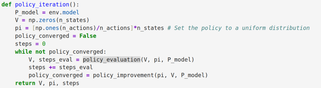
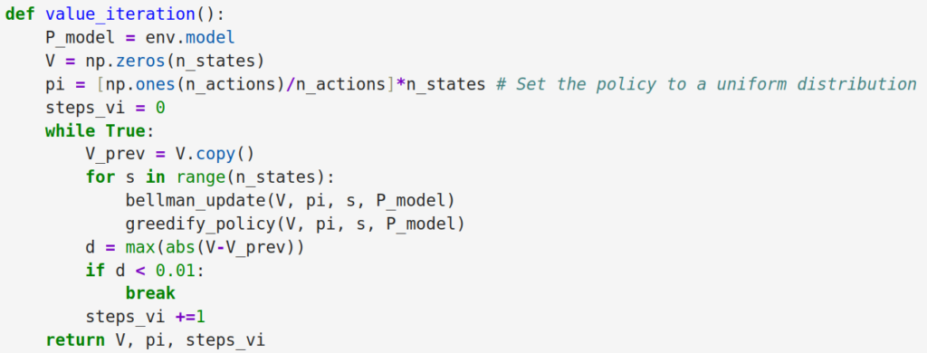
When we run a full policy evaluation (until convergence) and a full policy improvement (for every state) multiple times until both converge to stable values this is known as Policy Iteration. However, both value function and policy will converge even if we don’t update all of the value function or if we don’t run a full sweep of policy iteration; just a few steps are enough to guarantee that the two will eventually converge to their optimal values. This is the concept known as Generalized Policy Iteration (GPI). One extreme example of this is Value Iteration, were we only apply a single update of policy evaluation and improvement for each state.

Policy Iteration

As mentioned above, the Policy Iteration consists in running the Policy Evaluation until convergence multiple times (followed each time by a full sweep of Policy Improvement) until both the policy and the value function converge. This can be summarized by the following pseudo-code:

1. While policy and value not stable:
   • While value not stable:
     • update value function (Bellman update)
   • For each state:
     • Gredify policy

Value Iteration

Differently from Policy Iteration (PI), Value Iteration (VI) consists in running a single step of Policy Evaluation and Policy Improvement repeatedly until convergence of both. This is often faster than PI, as the value function is constantly updated with the latest policies. There is an alternative, implicit, way to perform value iteration, which will be shown later. In the mean time, here is the pseudo-code for VI in its explicit form:

1. While policy and value not converged:
   • For each state s:
     • update value function with Bellman update
     • Gredify policy

Bellman Optimality Equation

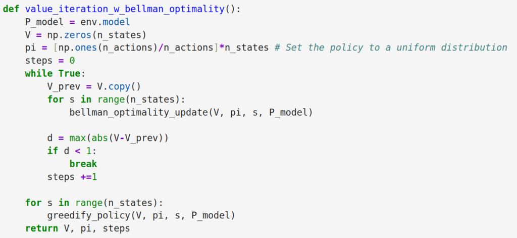
The “standard” Bellman equation evaluates a target policy \(\pi\); the Bellman Optimality equation, instead, evaluates the optimal policy \(\pi^*\). Instead of using \(a_{t+1} = \pi(s_t, a_t)\) as in Eq. (2), it uses \(a^* = argmax Q_{\pi^*}(s_t, a_t)\). It can be shown that \(Q_{\pi^*}(s_t, a^*) = max_{a} Q_{\pi^*}(s_{t+1}, a)\). The Bellman Optimality equation can, therefore, be written in the following form:

\begin{equation} Q_{\pi^*}(s_t, a_t) = \sum_{a_t \in \mathcal{A(s_t)}} \pi(a_t|s_t) \sum_{s_{t+1} \in \mathcal{S}} \sum_{r_t \in \mathcal{R}} p(s_{t+1}, r_t| s_t, a_t)[r + \gamma \cdot max_{a} Q_{\pi^*}(s_{t+1}, a)] \tag{3} \end{equation}

The BOE effectively merges the two steps of policy evaluation and improvement shown in Fig. 2. We can, therefore, come up with an implicit rule for Value Iteration that replaces the “bellman_update” and “greedify_policy” with a single step of “bellman_optimality_update”.

The Value Iteration implicit rule can be summarized as below:

1. While policy and value not converged:
   • For each state s:
     • update value function with Bellman Optimality update
2. For each state s:
   • Gredify policy

Code

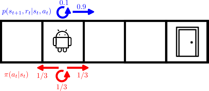
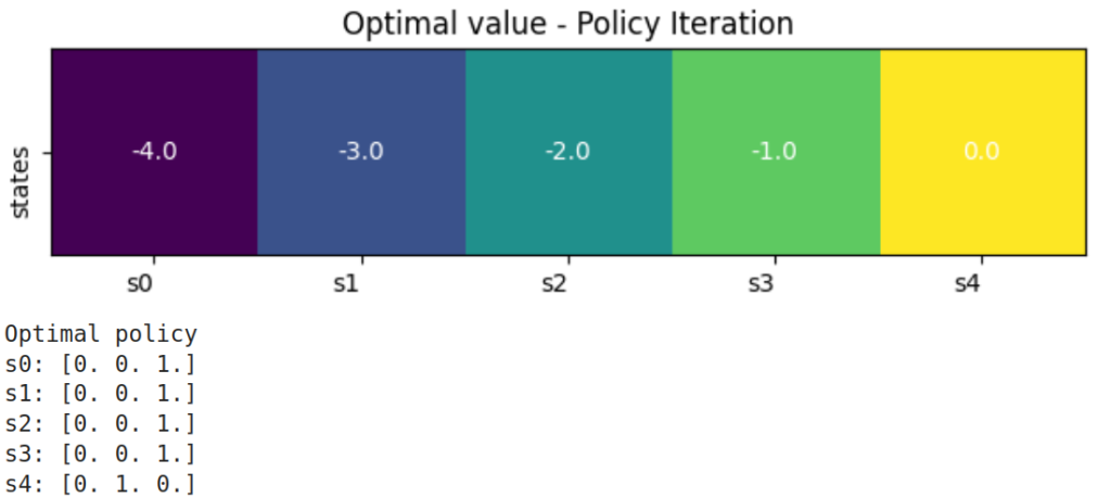
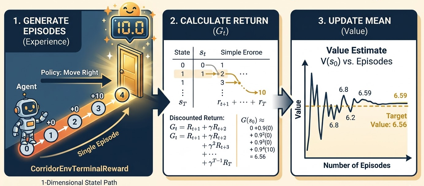
We have applied the algorithms shown above to the same Corridor Environment introduced in our previous post regarding Policy Evaluation. #

You can head to this Jupyter notebook where you will see that all the three variants of GPI (PI, VI-explicit and VI-implicit) all converge to the same optimal policy where the robot moves from left to right in order to reach the exit door as expected. You will notice, however, a big difference in terms of convergence steps, as PI takes many more steps to reach the optimal policy compared to both VI-implicit and VI-explicit. This is because, as mentioned above, VI updates its values with the latest policy, and therefore converges faster.

You can find a Jupyter Notebook in python to replicate the results above at this GitHub link.

References

• [1] R. S. Sutton and A. G. Barto, “Reinforcement Learning“, 2nd edition, 2015;
• [2] Fundamentals of Reinforcement Learning, Martha White and Adam White, visited Feb. 2025.
• [3] Grokking Deep Reinforcement Learning, Miguel Morales, book and github